3 Programming concepts
So far we have been working with the selfiesCasualties dataset knowing little about its nature and structure. However, a good understanding of R fundamentals is crucial to work effectively with R. Investing a good amount of time at learning about the R fundamentals arguably pays off in the long term, although new users might be prone to begin by hacking or artistically reusing code already available. This is a very short-sighted strategy, since you will find extremely hard to wrap your head around error messages, or cryptic default behavior such as the wrong definition of the y-axis in Figure 4.4. A good understanding of data structures instead, For instance, some functions accept only certain structures (e.g., dataframes 3.2.3, vectors 3.2.1) and data types (e.g., character, numeric), or their output might differ dending on the latters. For this reason, the goal of this chapter is to give you a set of tools to investigate the structure of objecst you work with. R is an object oriented language, which implise any time you run a function, its output will not permanently be stored in memory unless you assign it to an object. The way you assign content to objects is using the <- operator.
3.1 Functions
A function is an R object that performs an action on other R objects. In fact, R is object oriented, meaning that every element in as an object; functions make no exception since they are also objects in their own right. In fact, objects such as geom_bar from Chapter @:dataVisualization are nothing else but containers for instructions on what to when other objects (e.g., selfiesCasualties) are passed to an argument. In this training we are not covering custom functions, instead we either use functions from base R or the tidyverse suite (e.g., mean(), sum(), gather()). Use ? followed by the function to access the documentation, for instance by typing ?mean(). In particular, you want to learn about the parameters required for running a function and their format. Parameters cam be passed ordinally or by declaring the argumnent they are mapping to. For instace any vector passed to the function mean() will automatically be mapped to its x (first element). Note that apart from the minimum number of parameters required, functions might attribute default values to some other parameters (e.g., mean() has na.rm = FALSE). Make sure you undertsand what those default values imply by riding the documentation.
3.2 Data structures
3.2.1 Vectors
A vector is an adimensional collection of homogeneus elements, and the ultimate constitutive part of R data structures. To create a vector, use the function c() and comma-separate your elements.
It is R’s ultimate constitutive part, because R does not contemplate scalars, and even single numbers are ultimately vectors of length one, in fact:
is.atomic(1)## [1] TRUENote that is.vector() instead testes if the vector is a vector and has no other attributes than names. For instance:
is.atomic(factor(c('a')))## [1] TRUEis.vector(factor(c('a')))## [1] FALSESecond, vectors are homogeneus because all elements belong to the same datatype. Table 3.1 presents the four most relevant datatypes:
| code | typeof |
|---|---|
| c(‘1’,‘2’, ‘text’) | character |
| c(1L ,2L) | integer |
| c(1.5, 2.1) | double |
| c(TRUE, FALSE) | logical |
Categorical variables can be represented as an integer vector where each number corrisponds to a level. For instance, the vector:
factor(c('Pizza', 'Lasagne', 'Maccheroni'))## [1] Pizza Lasagne Maccheroni
## Levels: Lasagne Maccheroni Pizzacan be coherced to an integer using, with integer assigned by sorting the factor levels alphabetically:
as.integer(factor(c('Pizza', 'Lasagne', 'Maccheroni')))## [1] 3 1 2Third, vectors are adimensional:
dim(c(1, 10))## NULLTo subset a vector, use [ combined with a vector of the indexes you want to subest. Remember that in R the first element has index 1 (and not 0), thus to retrieve the 1st and the 3rd elements:
letters[c(1, 3)]## [1] "a" "c"You can also use indexing to overwrite elements or to append new ones, in combination with the assignment operator <-. For instance:
letters[c(1, 3)] <- c('New value', 'Another new value')
letters[c(1, 3)]
## [1] "New value" "Another new value"When appending a value to a position which falls out of bounds, R will fill the blanks up to that position with NA (missig values) without giving you any warnings. For instance letters has 26 elements, yet if we assign an element to position 100:
letters[100] <- 'position100'
length(letters)
## [1] 1003.2.2 Data types
As Table 3.1 shows, the way you pass elements in c() determine the type of your vector; e.g. numbers are interpreted as numeric values, while quoted elements become text strings. However, you can always convert an object type into another using the functions as.*. For instance, to coherce from character to double:
as.double( c('1', '3','20', '100'))## [1] 1 3 20 100Using the appropriate data type is crucial to avoid error and unexpected behaviors when running functions. For instance, from ?sort() we know that the argument x in sort() should be:
object with a class or a numeric, complex, character or logical vector.
Despite both numeric and character vectors are acceptable, using a character vector when we really want to order numbers is very misleading. In fact, if the vector of digits is stored as a character vector, sort() orders the values alphabetically:
sort(c('1', '3','20', '100', '5', '4'))## [1] "1" "100" "20" "3" "4" "5"3.2.3 Lists and dataframes
A data frame is the most readable structure for storing data, consisting in the columwise combination of vectors of equal length but any type. The dataset selfiesCasualties is an example of dataframe. Use str() to inspect its structure:
str(selfiesCasualties)## Classes 'tbl_df', 'tbl' and 'data.frame': 85 obs. of 7 variables:
## $ class : chr "Electricity" "Height" "Vehicles" "Vehicles" ...
## $ country : chr "Spain" "Russia" "USA" "USA" ...
## $ gender : Factor w/ 2 levels "Female","Male": 2 1 1 2 2 1 1 2 2 2 ...
## $ age : chr "21" "17" "32" "29" ...
## $ nationality: Factor w/ 24 levels "Australia","Bulgaria",..: 22 17 24 24 6 9 14 15 6 11 ...
## $ month : chr "March" "April" "April" "May" ...
## $ year : int 2014 2014 2014 2014 2014 2014 2014 2014 2014 2014 ...The very first line from the output shows that selfiesCausalties is of class data.frame, and has 85 observations (rows) and 7 variables (columns). In fact:
nrow(selfiesCasualties)## [1] 85ncol(selfiesCasualties)## [1] 7dim(selfiesCasualties)## [1] 85 7To select a variable from selfiesCasualties there are different options depending on the desired structure of the output. For example:
- to extract
age, namely to return a vector with the values of the variableage:$operatorselfiesCasualties$age(orselfiesCasualties$'age')[[operatorselfiesCasualties[['age']]
- to subset
age, namely to return a subset ofselfiesCasualtieswith only the variableage:[operatorselfiesCasualties['age']
Rows and columns could also be subset using positional indexing of the row-column combinations we wan to retrieve. For instance, to retrieve the first 10 records from columns 1 to 3:
selfiesCasualties[c(1, 10), 1:3]## # A tibble: 2 x 3
## class country gender
## <chr> <chr> <fctr>
## 1 Electricity Spain Male
## 2 Weapons Mexico MaleOr equivalently, we can combine positional and nominal indexing:
selfiesCasualties[c(1, 10), c('class', 'country', 'gender')]## # A tibble: 2 x 3
## class country gender
## <chr> <chr> <fctr>
## 1 Electricity Spain Male
## 2 Weapons Mexico MaleUnder the hood, a data frame is a special case of a list, where each element is a vector of equal length. In fact:
typeof(selfiesCasualties)## [1] "list"In a list, every element can have a different structure and dimensions.
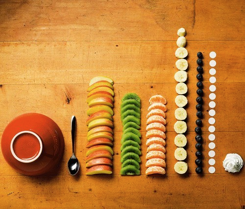
Figure 3.1: A cutboard with objects of different types, namely the best metaphorical representation of a list I could come up with
onTheTable <- list(dishes = 'milk cup',
                 cutlery = 'spoon',
                 appleWeight = sample(1:20, 15, T),
                 kiwiWeight = sample(1:20, 10, T),
                 mandarin = data.frame(sliceId = 1:10, weight = sample(1:20, 10, T)))
onTheTable
## $dishes
## [1] "milk cup"
##
## $cutlery
## [1] "spoon"
##
## $appleWeight
## [1] 12 1 12 2 4 11 6 9 10 6 4 17 16 19 5
##
## $kiwiWeight
## [1] 8 14 19 13 8 15 20 10 20 11
##
## $mandarin
## sliceId weight
## 1 1 12
## 2 2 8
## 3 3 13
## 4 4 16
## 5 5 15
## 6 6 11
## 7 7 8
## 8 8 2
## 9 9 1
## 10 10 15For example the object onTheTable contains both vectors of different lengths and a data frame; but virtually, each element could be another list containing more elements, and so forth.
To grasp the concept of list and how to index on these data structures is relevant because many functions (e.g. lm() for linear regression) output a list, which you might need to manipulate further. For instance, suppose we want to calculate the sum of squares from the following linear model:
fit <- lm(speed ~ dist, data = cars)
fit
##
## Call:
## lm(formula = speed ~ dist, data = cars)
##
## Coefficients:
## (Intercept) dist
## 8.2839 0.1656The residuals are stored in the element residuals within the object fit (a list). However, to extract the vector of the residuals, it is important to understand the difference between the [ and [[ operators. In fact:
sum(fit['residuals']^2)## Error in fit["residuals"]^2: non-numeric argument to binary operatorBecause fit['residuals'] subsets the list, but does not extract the numeric vector inside the list itself. In fact:
str(fit['residuals'])## List of 1
## $ residuals: Named num [1:50] -4.62 -5.94 -1.95 -4.93 -2.93 ...
## ..- attr(*, "names")= chr [1:50] "1" "2" "3" "4" ...Instead, to extract an element (in this case a vector) from fit you need [[:
sum(fit[['residuals']]^2)## [1] 478.02123.2.4 Tibbles
Tibble is a recent data structure that combines the flexibility of lists (different structures in the same object), with the readability of dataframes (keep data in a rectangular format). Tibbles are easier to manipulate using tidyverse, in particular when working with dplyr and purrr (Chapter 5. To transform a data.frame into a tibble:
selfiesCasualties <- as_data_frame(selfiesCasualties)
selfiesCasualties
## # A tibble: 85 x 7
## class country gender age nationality month year
## <chr> <chr> <fctr> <chr> <fctr> <chr> <int>
## 1 Electricity Spain Male 21 Spain March 2014
## 2 Height Russia Female 17 Russia April 2014
## 3 Vehicles USA Female 32 USA April 2014
## 4 Vehicles USA Male 29 USA May 2014
## 5 Train India Male 15 India May 2014
## 6 Height Italy Female 16 Italy June 2014
## 7 Height Philippines Female 14 Philippines July 2014
## 8 Height Portugal Male unknown Poland August 2014
## 9 Electricity India Male 14 India August 2014
## 10 Weapons Mexico Male 21 Mexico August 2014
## # ... with 75 more rowsNote that:
class(selfiesCasualties)## [1] "tbl_df" "tbl" "data.frame"which means that tibbles are also data frames, but they can accomodate column-lists too, instead of column-vectors only. For instance:
tib <- tibble(Values = list(1:10, 1:5),
          SequenceName = c('First sequence', 'Second sequence'))
tib
## # A tibble: 2 x 2
## Values SequenceName
## <list> <chr>
## 1 <int [10]> First sequence
## 2 <int [5]> Second sequencestr(tib)## Classes 'tbl_df', 'tbl' and 'data.frame': 2 obs. of 2 variables:
## $ Values :List of 2
## ..$ : int 1 2 3 4 5 6 7 8 9 10
## ..$ : int 1 2 3 4 5
## $ SequenceName: chr "First sequence" "Second sequence"3.3 Logical and Mathematical Operators
Logical and mathematical operators are extremely useful conditioanl operations, such as indexing. Logical operators follows mathematical logic and are:
!NOT&AND|OR
Mathematical operators instead:
==indicates equality (note that=is equivalent to<-instead)>=at least or<=no bigger than>strictly bigger<strickly smaller
Other logical operators:
- %in% matching values
For example, to retrieve a subset of males who died in a foreign country (namely their nationality is not from the country they died in):
selfiesCasualties[selfiesCasualties$gender=='Male' & selfiesCasualties$country!=selfiesCasualties$nationality,]## # A tibble: 7 x 7
## class country gender age nationality month year
## <chr> <chr> <fctr> <chr> <fctr> <chr> <int>
## 1 Height Portugal Male unknown Poland August 2014
## 2 Train India Male 24 Israel February 2015
## 3 Height Indonesia Male 21 Singapore May 2015
## 4 Height India Male unknown Japan September 2015
## 5 <NA> <NA> <NA> <NA> <NA> <NA> NA
## 6 Height Peru Male 28 South Korea June 2016
## 7 Height Peru Male 51 Germany June 2016Keep in mind that logical comparisons of vector elements require a single logical operator (&, | or !), whereas a double operator (e.g., &&) compares only the first element of two vectors.
With operations that resolve to a logical value, dealing with NA might become tricky because of how R handles NA. In fact NA is not a zero, but a placeholder for a missing value. With logical operators, R retrieves an NA any time that the result is ambiguous, but a logical value when the output is certain regardless than NA.
| code | output |
|---|---|
| TRUE & NA | NA |
| FALSE | NA | NA |
| NA == NA | NA |
| FALSE & NA | FALSE |
| TRUE | NA | TRUE |
With mathematical operators instead, the results is always NA. Thus, to test whether a value equals NA we use is.na() instead of ==.